Circos流程记录
最近要用到Circos进行绘图,因此进行记录,方便下次绘图。
0. 软件安装
Circos基于Perl,所以我们需要进行大量Perl包的安装。当然,秉着赌狗的心理,我们看看能不能直接通过conda装。
# conda新建名为 Circos 的环境(每次安装独立的软件时,都建议新建一个conda环境安装,不容易出现什么安装冲突)
conda create -n Circos
# 激活环境
conda activate Circos
# 通过bioconda源搜索circos,看看有哪些版本
conda search circos -c bioconda
# 这里我们安装最新的 0.69.9
conda install circos=0.69.9 -c bioconda
# 这里没有报错,直接输入 y 进行安装
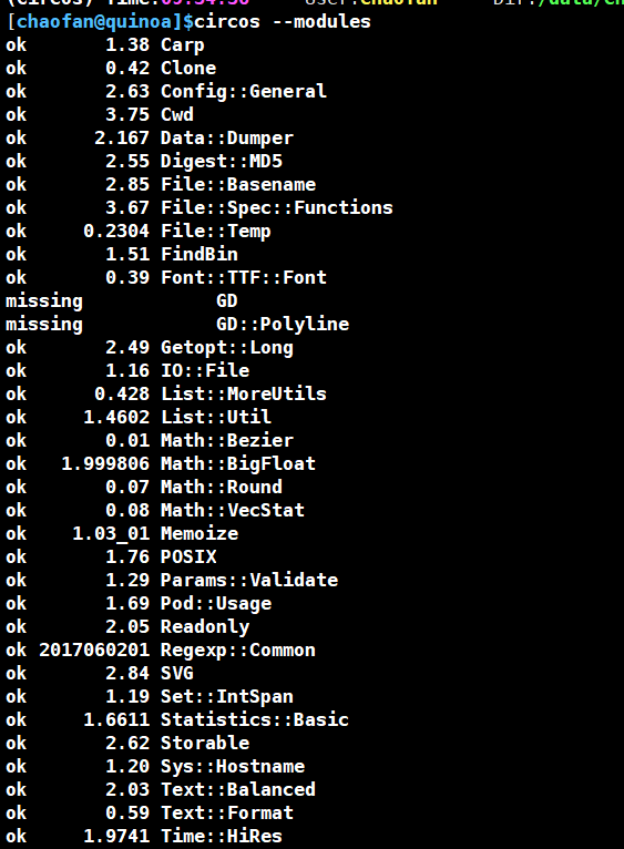
# conda安装后 检查是否有依赖缺失
circos --modules这里我们缺少GD和GD::Polyline模块。
# 通过 conda 安装 libgd 依赖
conda install -c fastchan libgd

# 通过 conda 安装 perl-gd (perl的gd模块)
conda install -c bioconda perl-gd

# 如果libwebp这个版本装不上,就直接把版本号去掉安装,然后在conda这个环境的lib文件夹下 "骗软件"
# ln -s libwebp.so.7 libwebp.so.6
conda install -c conda-forge libwebp=0.5.2

# 最后检查一遍,一般help文档能出来就说明装成功了
circos -h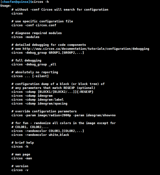
1. Circos的使用
1.1 绘制染色体(karyotype)
我们首先需要准备一个karyotype文件,这个文件描述了所绘制染色体的基本信息。这个文件由七列构成,无表头,任意空白字符分割即可。
faidx ../nextDevono.fa -i chromsizes | sort -nr -k2 | awk '{print "chr", "-", $1,NR,"0",$2, "169,69,255"}' > karyotype.txt

faidx /data/chaofan/projects/06.daily/20.Alternata_gff/04.final_res/Z7.fa -i chromsizes | sort -n -k2 | awk '{print "chr", "-", $1,13-NR,"0",$2, "6,97,118"}' >> karyotype.txt
这里我们的结果文件如下所示:
karyotype.txt# 这里前两列是karyotype固定的,代表绘制染色体
# 第三列是染色体ID,也是其他配置文件的坐标锚点
# 第四列是具体展示在图上的染色体名称
# 第五、六列是染色体起始、终止位置 起着展示染色体长度的信息
# 第七列则是染色体方块的颜色,这里名称为RGB颜色
chr - ctg000130 1 0 6741225 169,69,255
chr - ctg000050 2 0 5683444 169,69,255
chr - ctg000120 3 0 3309307 169,69,255
chr - ctg000020 4 0 3201804 169,69,255
chr - ctg000100 5 0 2838009 169,69,255
chr - ctg000040 6 0 2659068 169,69,255
chr - ctg000030 7 0 2635818 169,69,255
chr - ctg000110 8 0 2444020 169,69,255
chr - ctg000010 9 0 2417686 169,69,255
chr - ctg000000 10 0 1868462 169,69,255
chr - ctg000090 11 0 561846 169,69,255
chr - ctg000070 12 0 75900 169,69,255
chr - ctg000080 13 0 72450 169,69,255
chr - ctg000060 14 0 61073 169,69,255
chr - 12 12 0 416412 6,97,118
chr - 11 11 0 561391 6,97,118
chr - 10 10 0 1841737 6,97,118
chr - 9 9 0 2401432 6,97,118
chr - 8 8 0 2464928 6,97,118
chr - 7 7 0 2519108 6,97,118
chr - 6 6 0 2544158 6,97,118
chr - 5 5 0 2863349 6,97,118
chr - 4 4 0 3085453 6,97,118
chr - 3 3 0 3269484 6,97,118
chr - 2 2 0 5542836 6,97,118
chr - 1 1 0 6770053 6,97,118
我们先生成一个染色体的配置文件ideogram.conf,将以下内容放到这个文件中,展示我们上面生成的染色体形状。
ideogram.conf#指定染色体文件(绝对/相对路径+文件名)
##########################################################################
<ideogram>                #这是定义染色体相关参数的标签,相当于HTML的一个条目
<spacing>                 #定义染色体间隙宽度的标签,以</spacing>,其中包括要设置的参数
default = 0.006r          #r指的是圆的周长,设置0.5%圆的周长为间隙
<pairwise 1;ctg000130>       #可以用<pairwise>标签特别指定某些染色体的间隙(用的是ID),因为在大多数文章中,都会留一个大间隙,来放label
spacing = 5r            #这里20r表示是相对default = 0.005r的20倍,也就是10%的圆的周长
</pairwise>              #标签都要以</>结尾,
<pairwise 12;ctg000060>
spacing = 5r
</pairwise>
</spacing>                #间隙定义结束,下面是对染色体样式的调整

radius           = 0.65r  #轮廓的位置,这里的r指的是半径,由圆心到圆周上范围依次是0-1r,,超出部分将不再显示。
thickness        = 20p    #染色体整体的宽度,这里p指的是像素大小,也可以用r表示,1r=1500p
fill             = yes    #是否为染色体填充颜色,如果为yes,自动用第七列定义的颜色着色
stroke_color     = dgrey  #染色体边框的颜色,支持多种格式的输入,如:red或255,182,106
stroke_thickness = 2p     #染色体边框的粗细

show_label     = yes # 展示染色体ID
label_with_tag = yes # tag 标识是否包含到 label 中
label_font     = bold # label 的字体
label_center   = yes
label_size     = 32p
label_color    = grey
label_parallel = yes # label方向, 是否与圆外圈平行
label_case     = upper # label 的大小写:upper,lower
label_radius = 0.98r

</ideogram>               #定义染色体属性的标签结束
##########################################################################
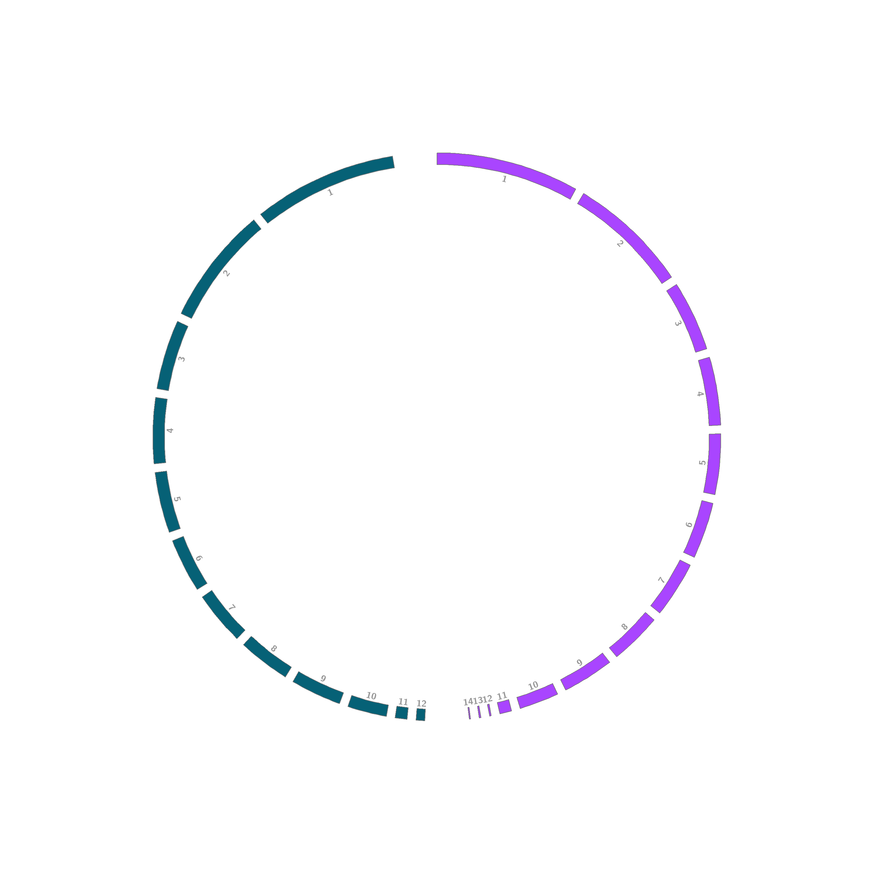
我们再配置一个基础的运行conf文件: Alternaria.conf
Alternaria.conf##########################################################################
chromosomes_units           = 100000 # 设置u的单位,1u = 100kbp

karyotype = ./karyotype.txt
<<include ideogram.conf>>

#下面是每次都要复制粘贴上去的,他们属于circos自带的配置文件,用于调用颜色,距离,报错等信息
<image>                    #注意路径
<<include etc/image.conf>> #注意引用外部配置文件需要使用<<#>>
</image>
<<include etc/colors_fonts_patterns.conf>>
<<include etc/housekeeping.conf>>
##########################################################################
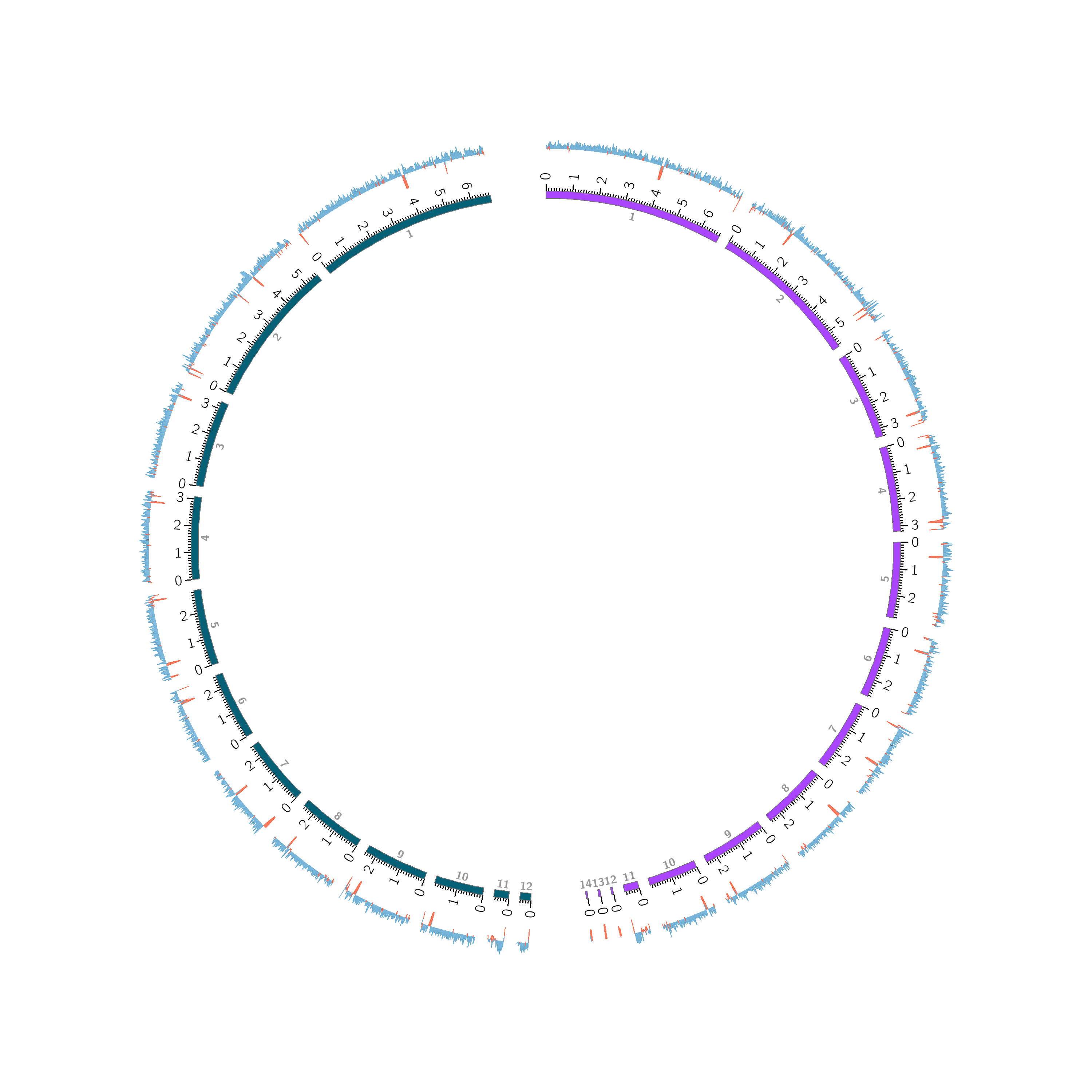
circos -conf Alternaria.conf我们得到了初步的染色体结果:
我们再配置一个ticks.conf文件,加上染色体ID及刻度线。
ticks.conf##########################################################################
# 配置染色体标签和刻度线
show_ticks          = yes  #选择yes表示要显示刻度线
show_tick_labels    = yes  #选择yes表示要显示刻度线的数值
#定义刻度线的整体位置与形状
<ticks>                    #刻度线的转用标签,但凡是复数出现的,其下面的参数都表示全局参数,像下面的<tick>单数形式,都表示局部参数
radius           = 1r      #刻度线的位置,1r为最远距离,超过1r不再显示
color            = black
thickness        = 3p
multiplier       = 1e-6    #刻度标签的大小,这里我们一个标签=10u,这里大刻度就是1=1M,如果multiplier=1e-5,那这里的刻度就是10
format           = %d      #然后以整数的形式标记在刻度线上
#定义小的刻度线,且不显示数值
<tick>
spacing        = 1u        #最开始我们定义1u = multiplier = 100000,表示一个小刻度为100kbp
size           = 8p
show_label     = no        # 是否展示小刻度线
</tick>
#定义大的刻度线,显示数值
<tick>
spacing        = 10u # 这里设置一个大刻度为10个小刻度
size           = 20p
show_label     = yes
label_size     = 30p
label_offset   = 10p      #设置数值和刻度线之间的间隔
format         = %d
</tick>
</ticks>
##########################################################################
我们再在Alternaria.conf中加入这个ticks.conf
Alternaria.conf##########################################################################
chromosomes_units           = 100000 # 设置u的单位,1u = 100kbp

karyotype = ./karyotype.txt
<<include ideogram.conf>>
<<include ticks.conf>>


#下面是每次都要复制粘贴上去的,他们属于circos自带的配置文件,用于调用颜色,距离,报错等信息
<image>                    #注意路径
<<include etc/image.conf>> #注意引用外部配置文件需要使用<<#>>
</image>
<<include etc/colors_fonts_patterns.conf>>
<<include etc/housekeeping.conf>>
##########################################################################
# 运行
circos -conf Alternaria.conf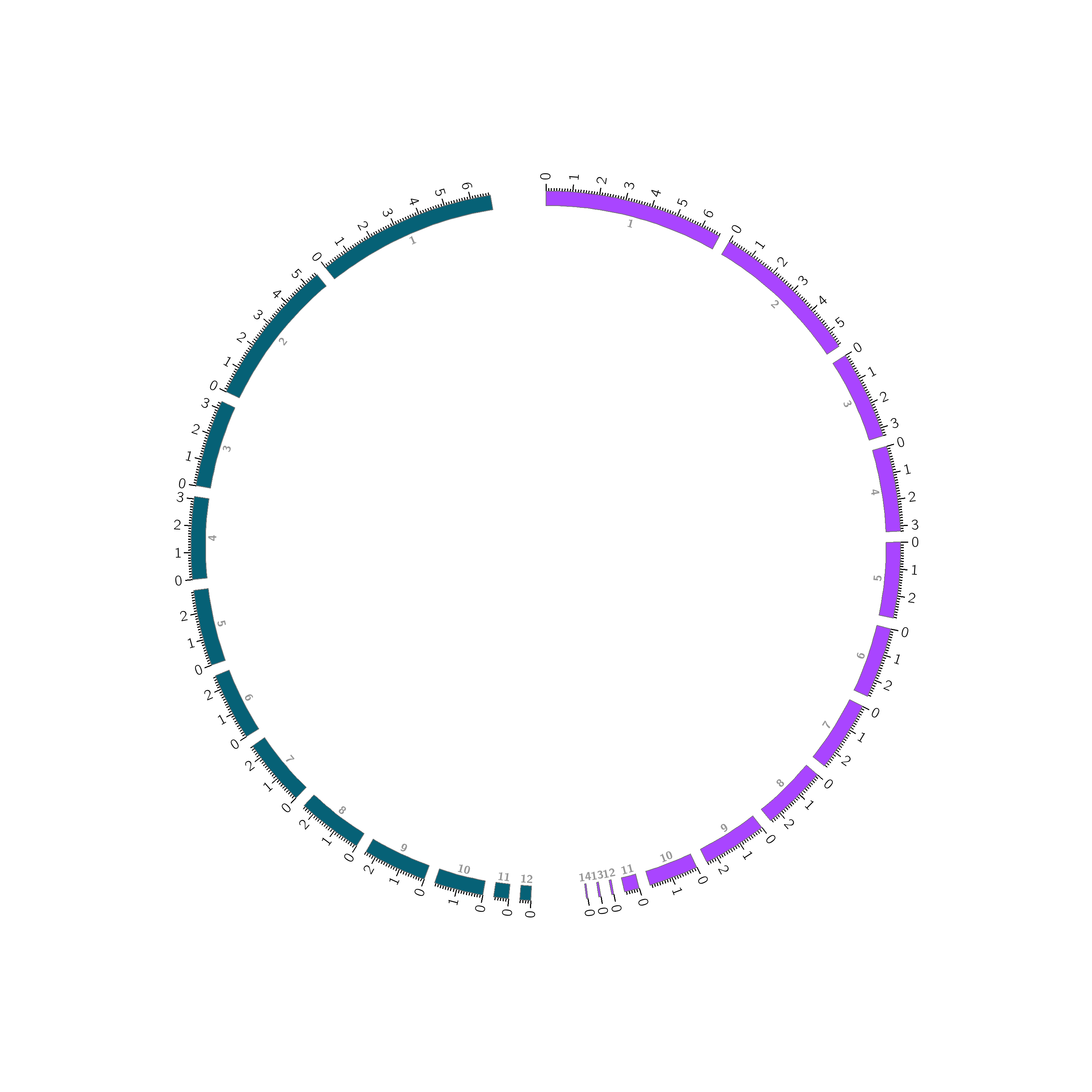
1.2 外圈展示GC含量
faidx ../nextDevono.fa -i chromsizes >  nextDevono.txt
faidx /data/chaofan/projects/06.daily/20.Alternata_gff/04.final_res/Z7.fa -i chromsizes >  Z7.txt

bedtools makewindows -g nextDevono.txt -w 20000 > gaisen.20kb.win
bedtools makewindows -g Z7.txt -w 20000 | sort -n -k 1 -n -k 2  > Z7.20kb.win

bedtools nuc -fi ../nextDevono.fa -bed gaisen.20kb.win | \
cut -f 1-3,5 | grep -v "#" | \
awk -vFS="\t" -vOFS="\t" '{print $1,$2,$3,$4*(100)-50}' > gc.density.txt

bedtools nuc -fi /data/chaofan/projects/06.daily/20.Alternata_gff/04.final_res/Z7.fa -bed Z7.20kb.win | \
cut -f 1-3,5 | grep -v "#" | \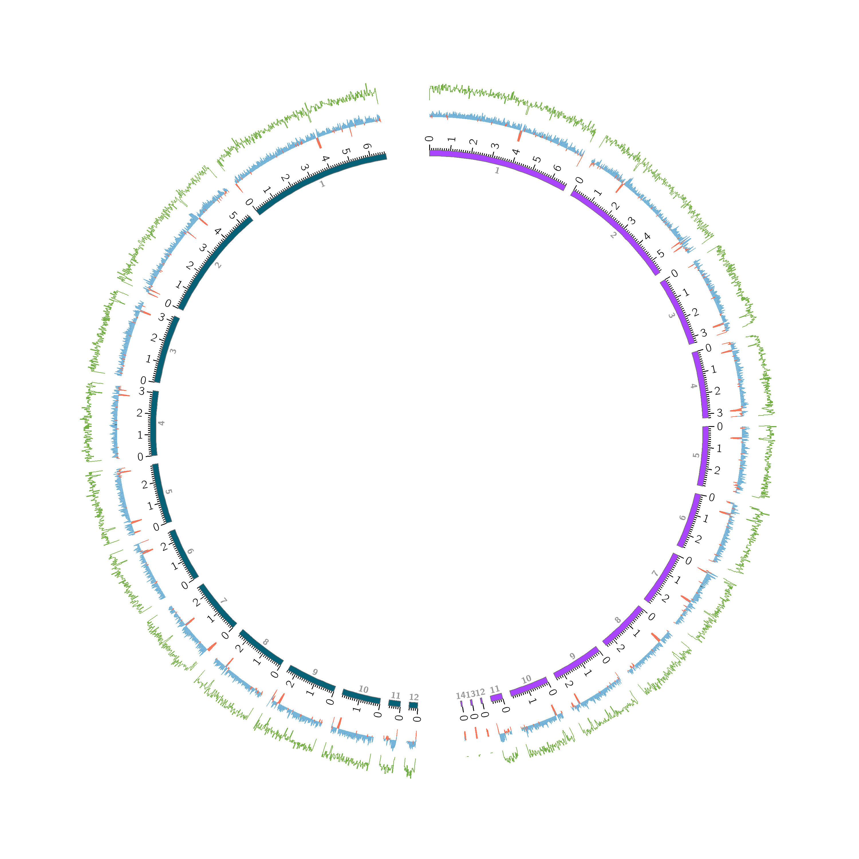
awk -vFS="\t" -vOFS="\t" '{print $1,$2,$3,$4*(100)-50}' >> gc.density.txt我们另外生成一个GC.conf文件。
GC.conf<plots>
    <plot>
        type      = line #设定显示类型
        thickness = 2p #折线图的粗细
        max_gap = 1u
        file    = gc.density.txt #输入数据
        color   = vdgrey #折线颜色
        min     = -5 #环道内圈代表的数值下限,超出下限的数值不会显示,下同
        max     = 5 #环道外圈代表的数值上限
        r0      = 1.06r #环道内圈位置
        r1      = 1.18r #环道外圈位置

        fill_color = vdgrey_a3
        <rules>
            <rule> #设置折线图大于0部分显示为蓝色
                condition    = var(value) > 0
                color        = blue
                fill_color   = blue_a1
            </rule>

            <rule> #设置折线图小于0部分显示为红色
                condition    = var(value) < 0
                color        = red
                fill_color   = red_a1
            </rule>
        </rules>
    </plot>
</plots>
1.3 外圈展示基因含量
grep '[[:blank:]]gene[[:blank:]]' ../fungap_out.gff3 | \
awk '{print $1"\t"$4"\t"$5}' |
bedtools coverage -a gaisen.20kb.win -b - | \
cut -f 1-4 > gene.density.txt

grep '[[:blank:]]gene[[:blank:]]' /data/chaofan/projects/06.daily/20.Alternata_gff/04.final_res/2023-10-05.corrected.gff3 | \
awk '{print $1"\t"$4"\t"$5}' |
bedtools coverage -a Z7.20kb.win -b - | \
cut -f 1-4 >> gene.density.txt我们把gene_density信息也加到GC.conf文件。
GC.conf<plots>
    <plot>
        type      = line #设定显示类型
        thickness = 2p #折线图的粗细
        max_gap = 1u
        file    = gc.density.txt #输入数据
        color   = vdgrey #折线颜色
        min     = -5 #环道内圈代表的数值下限,超出下限的数值不会显示,下同
        max     = 5 #环道外圈代表的数值上限
        r0      = 1.08r #环道内圈位置
        r1      = 1.16r #环道外圈位置

        fill_color = vdgrey_a3
        <rules>
            <rule> #设置折线图大于0部分显示为蓝色
                condition    = var(value) > 0
                color        = blue
                fill_color   = blue_a1
            </rule>

            <rule> #设置折线图小于0部分显示为红色
                condition    = var(value) < 0
                color        = red
                fill_color   = red_a1
            </rule>
        </rules>
    </plot>
    ########################################## NEW ##########################
    <plot>
    type      = histogram #设定显示类型
    thickness = 2p #折线图的粗细
	file = gene.density.txt
	r0 = 1.18r
	r1 = 1.26r
	color = 114,176,67
    </plot>
    ########################################## NEW ##########################
</plots>
1.4 展示共线性基因
我们首先通过JCVI鉴定两个基因组上的共线性区域,通过simple文件提取共线性区域。
python -m jcvi.formats.gff bed --type=mRNA --key=ID Gaisen.gff > Gaisen.bed

python -m jcvi.formats.gff bed --type=mRNA --key=ID Z7.gff > Z7.bed

# 鉴定两个基因组间的共线性基因
python -m jcvi.compara.catalog ortholog --dbtype prot Z7 Gaisen --cscore=.98 --no_strip_names

# 创建simple文件
python -m jcvi.compara.synteny screen --minspan=25 --simple Z7.Gaisen.anchors Z7.Gaisen.simple

# 从gff文件中提取simple block的区间
python jcvi2link.py /data/chaofan/projects/06.daily/20.Alternata_gff/04.final_res/2023-10-05.corrected.gff3 ../fungap_out.gff3 /data/chaofan/projects/06.daily/06.yelu/07.genome_assemble/07.JCVI/Z7.Gaisen.simple link.txt
jcvi2link.pyfrom sys import argv,exit


def gene_dic(gff):
    tmp_dic = {}
    for line in open(gff):
        if line[0] in ["#", "\n"]:
            continue

        tmp = line.strip().split("\t")
        if tmp[2] == "mRNA":
            tmp_dic[tmp[8].split(';')[0].split('=')[1]] = [tmp[0], int(tmp[3]), int(tmp[4])]

    return tmp_dic


if __name__ == '__main__':
    if len(argv) != 5:
        exit(f"python {argv[0]} [Z7_gff] [Gaisen_gff] [simple_file] [link_txt]")

    Z7_dic = gene_dic(argv[1])
    Gaisen_dic = gene_dic(argv[2])
    colors = {"+":"62,169,8","-":"65,182,230"}
    ouf_w = open(argv[4], "w")
    for line in open(argv[3]):
        tmp = line.strip().split("\t")
        Z7_min = min(Z7_dic[tmp[0]][1], Z7_dic[tmp[1]][1])
        Z7_max = max(Z7_dic[tmp[0]][2], Z7_dic[tmp[1]][2])

        Gaisen_min = min(Gaisen_dic[tmp[2]][1], Gaisen_dic[tmp[3]][1])
        Gaisen_max = max(Gaisen_dic[tmp[2]][2], Gaisen_dic[tmp[3]][2])
        ouf_w.write(Z7_dic[tmp[0]][0]+"\t"+str(Z7_min)+"\t"+str(Z7_max)+"\t"+Gaisen_dic[tmp[2]][0]+"\t"+str(Gaisen_min)+"\t"+str(Gaisen_max)+"\tcolor="+colors[tmp[5]]+"\n")

    ouf_w.close()
得到这样的结果文件: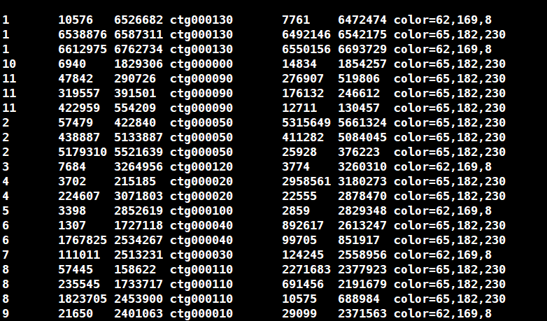
我们再配置link.conf文件:
link.conf<links>

<link>
file          = link.txt
ribbon        = yes
radius        = 0.95r
bezier_radius = 0r
flat   = yes # 强制条带不扭转
bezier_radius_purity = 0.5
thickness     = 1
</link>

</links>
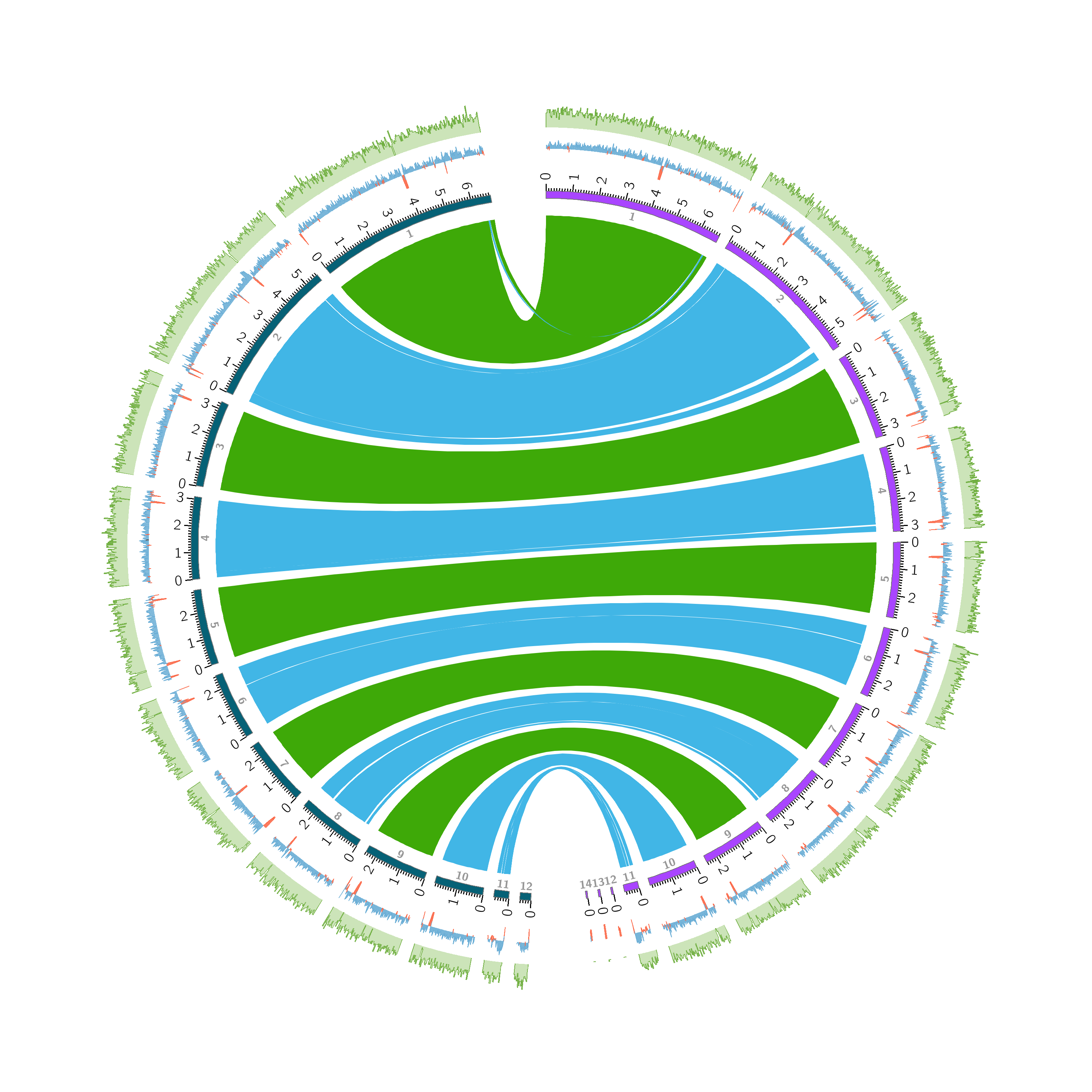
当然,还有很多进阶的配置,后面慢慢改。